Introduction to optical observations

This page summarizes important concepts concerning observations in optical astronomy, gives definitions that are essential to understanding the tutorial, and touches some very practical points. It’s kept as short as possible.

Telescope optics

A reflecting telescope uses a combination of (curved) mirrors to form an image in its so-called focal plane, also known as the image plane. The optical design of the AIfA telescope is a variation of a Cassegrain telescope, illustrated below.

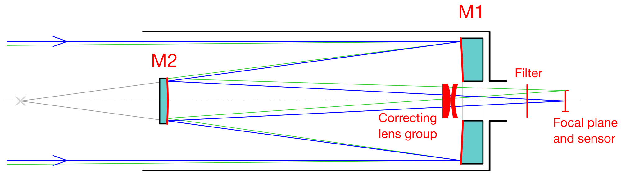
Fig. 1 Optical layout of the AIfA telescope

The in-falling light first meets the concave primary mirror (M1) to be then re-reflected by the convex secondary mirror (M2). The light gets collimated in the focal plane, after passing through an opening in M1. Due to the folding of its optical path, such a Cassegrain system allows for a compact construction. More precisely, the AIfA telescope is a “corrected Dall-Kirkham” telescope, where M1 is ellipsoidal with a diameter of 35 cm (the aperture of the telescope), M2 is spherical, and an additional lens group located before the focal plane, roughly in the opening of M1, corrects the design against aberrations on a wide and flat focal plane. The effective focal length of the system is 2563 mm.

Resolution

Due to diffraction, a telescope has a finite angular resolution. Note that this notion of resolution is not related to the sampling by a camera (i.e., pixel size), discussed later. Instead, it is a fundamental property of the optical system.

The light distribution in the image plane resulting from an (apparently) point-like source (star) is termed point-spread function (PSF). In the idealised (so-called diffraction-limited) case, the PSF of a circular aperture is given by the Airy disc. Using the Rayleigh criterion for spatial resolution, a telescope of primary aperture \(D\) at a wavelength \(\lambda\) is in principle capable of resolving structure with an angular separation (in radians) of

\[ \Delta \theta = 1.22 \frac{\lambda}{D}. \]

Question

What’s the diffraction-limited angular resolution of a telescope with an aperture of 35 cm, at a wavelength of 700 nm, in arcseconds?

As we’ll see in the following, for simple ground-based telescopes, the actual resolution will be lower, due to the effects of Earth’s atmosphere.

Seeing and airmass

For ground-based astronomical observations, Earth’s atmosphere has to be considered as part of the optical system, leading to numerous effects. Our atmosphere is inhomogeneous in temperature (and hence density), resulting in an inhomogeneous refractive index. Turbulence in the atmosphere leads to variations of this refractive index on short spatial and temporal scales. In consequence, the “instantaneous” image of a star seen in the telescope is no longer an Airy disc, but has a very irregular shape (see Speckle imaging for an example). Due to the fast temporal variation of the turbulent atmosphere, the star’s image randomly changes and moves around. Integrating this image with any exposure time longer than about a tenth of a second results in a blurry blob, which is wider than the diffraction-limited Airy disk. This ground-based PSF of a long exposure can to some extent be represented by a two-dimensional Gaussian. An even better approximation is given by the Moffat profile.

The size of such a stellar image, as given by the full width at half maximum (FWHM) of the PSF profile, is called the seeing of the image and measures the actual resolution in a particular observation. The less turbulent the atmosphere, the higher the resolution and thus the data quality that can be achieved. For Bonn, a seeing of 2 arcsec is a very rare and good value, while in excellent locations like Hawaii or the Atacama desert 0.5 arcsec are common.

Hint

Both the diffraction-limited resolution of a telescope and the seeing are wavelength-dependent! The diffraction-limited image is sharpest for shorter wavelength. But as just discussed, atmospheric seeing is a consequence of refraction. Refraction of visible light in the atmosphere (that is a medium with so-called “normal dispersion”) is stronger for short wavelengths than it is for long wavelengths. Therefore, a ground-based image taken in red (or infrared) light will be sharper than an image in the blue part of the spectrum (assuming otherwise similar observing conditions)!

The best possible observing conditions are achieved near the zenith, where the length of the light path through the atmosphere is minimal. Extinction and disturbing seeing effects get worse for observations at lower elevations. These effects are often expressed in terms of the object’s airmass \(a\), which tells you through how much atmosphere (column density) the light travels compared to vertical in-fall. For an angular distance \(z\) from the zenith (zenith = in vertical direction from the ground) it can in good approximation be computed as \(a = 1 / \cos(z)\) such that \(a = 1\) for an object at the zenith and formally \(a = \infty\) at the horizon.

Imaging instrument: the camera

A camera is an instrument attached to the telescope, such that the camera’s imaging sensor (sometimes also called detector) lies in the focal plane of the telescope. The sensor in the camera will sample the image, by recording the intensity of the light in an array of pixels (short for picture elements).

The combination of a camera with a telescope yields a particular size of the field of view, and a resulting pixel scale. The pixel scale corresponds to the angular size a pixel subtends on the sky, and is expressed in arcseconds. For example, the camera used at the 35 cm AIfA telescope has a field of 48 arcmin by 32 arcmin, and a pixel scale of 0.3 arcsec. Given how small these pixels are compared to the typical seeing, we systematically operate the camera with a “2x2 binning”, meaning in this particular case that adjacent pixels are summed together in groups of 2x2 pixels, with the benefit of reduced file size. The effective pixel size of those images is 0.607 arcsec.

Filters

While the sensors used in optical astronomy can virtually count individual photons, they are not sensitive to their wavelength. Therefore, to obtain any kind of color information, one has to record several images of the target using different optical filters. These filters are inserted in the optical path before the imaging sensor (see Fig. 1). In practice, several filters are mounted into a filter wheel which is located directly ahead of the camera, allowing for a fast filter change.

The filter wheel of the AIfA telescope contains broad-band filters that are very close to the ones used in the the Sloan/SDSS photometric system (called ugriz), which is widely used in astronomical research:

• g’ with a passband of about 400 - 550 nm (blue to green), very similar to SDSS g,

• r’ with a passband of about 560 - 700 nm (yellow to red), very similar to SDSS r,

• i’ with a passband of about 700 - 840 nm (red and near infrared), very similar to SDSS i.

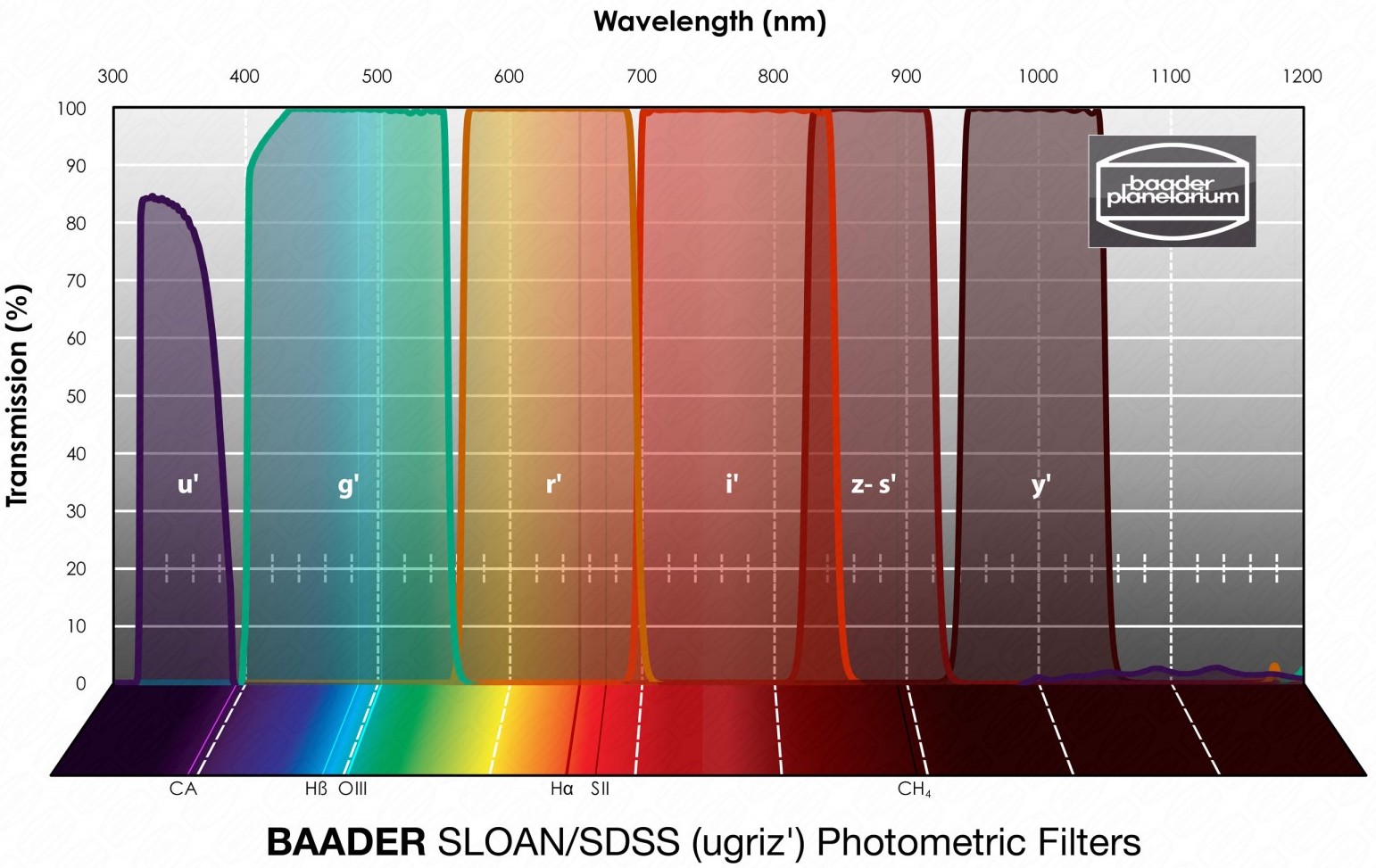
Fig. 2 Transmission curves of the photometric filters used at the AIfA telescope. Image credit: Baader Planetarium (manufacturer of our filters).

In addition, the filter wheel also holds three narrowband filters: H-alpha, OIII, and SII, each with a width of 6.5 nm.

Imaging detectors (CCD or CMOS)

Modern optical cameras use electronic sensors: the incoming photons create free electrons in silicon, and these free electrons are collected in potential wells, before being read out once the desired exposure time is completed. Two types of sensors for optical astronomy cameras are CCD and CMOS chips. A key difference between these is about where and how the collected charges in each pixel are amplified and converted to a digital signal: for the CCD, many pixels are read out by a single amplifier one after the other (with the charges of these pixels being transferred pixel to pixel towards the amplifier), while for the CMOS, each pixel has its own amplifier directly attached to it.

Historically, CCDs where better suited for astronomical imaging (mainly due to lower noise and higher sensitivity). Hence, most of the literature on astronomical image reduction is about CCDs. But CMOS sensors have now caught up for many applications, and the camera used at the AIfA telescope uses a modern CMOS sensor. In the scope of this tutorial, we will pass over the rather minor differences in the optimal processing of CCD or CMOS data. The general ideas that we will implement can be equally applied to both detectors.

We now describe some nomenclature as well as important aspects of these sensors. These are equally applicable to both types.

Quantum efficiency

The quantum efficiency (QE) is the ratio of electrons to the number of photons hitting the pixel. QEs of top grade sensors used in professional observatories are far above 90% over a significant wavelength range. For many basic considerations we can therefore assume that one photon leads to one electron, and use the words photons and electrons interchangeably. We will do so in the present tutorial.

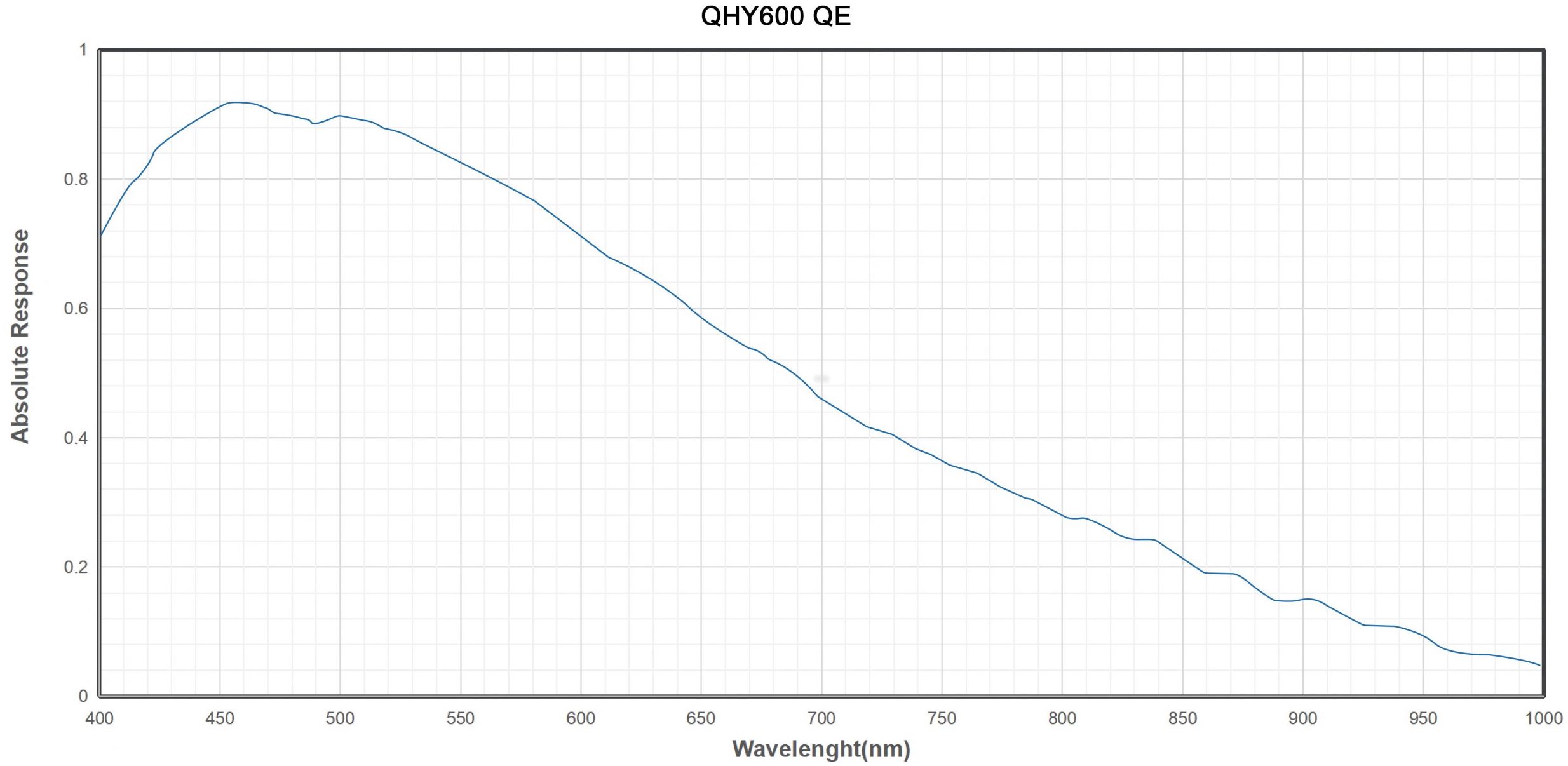
Fig. 3 Quantum efficiency curve of the QHYCCD 600M PH camera used at the AIfA telescope. The sensor is a Sony IMX455. Image credit: QHYCCD (manufacturer of the camera).

Full-well capacity

The charge capacity of a pixel is limited. The maximum number of electrons fitting into a single pixel is called full well capacity or simply “full well”. Typical scientific sensors have a full well of the order of \(10^5\) electrons. If the charge level is approaching full well the signal is getting non-linear and charges may spill over into adjacent pixels. Note that the full-well capacity is a physical property of the sensor’s pixels, and not just a “software issue” about how the pixel values are stored in a computer.

ADC, ADU, and gain

After the exposure, the electrons captured in a pixel get amplified, and the resulting potential is then converted to a digital number (the pixel value) by an electronic circuit called Analog-to-Digital Converter (ADC). For clarity, one attaches a “unit” to these digital numbers: pixel values are quoted in ADU, which is an acronym for Analog to Digital Unit. It is important to distinguish ADUs and numbers of electrons: these are different values! One defines the gain of the detector as the differential change in charge that produces a change of one ADU. In other words, this gain can be seen as the conversion factor between electrons and ADU (assuming an idealized detector with constant gain). This gain is set by the amplifier and the ADC. For our imaging camera at the AIfA telescope, the gain is 0.376 e/ADU when using our default settings (see the page Camera characterization if you’re interested in how this can be measured).

Bit depth

The bit depth is the number of bits used to express pixel values. It is a property of the ADC, and later of the image file. For example, a common ADC with 16 bits (unsigned) gives \(2^{16} = 65536\) (positive) integer values. The gain of an ADC is usually adjusted so that ADC saturates in the linear regime of the CCD, before the full-well capacity is reached. In this way, when we observe a pixel to have a value lower than 65536 ADU, we can be sure that we did not saturate the charge capacity of that pixel.

Note that raw images have integer pixel values. Once we process these images, we typically use floats.

Bias level

The bias level or simply bias is a small negative potential added by the electronics before the analog-to-digital conversion. This bias is needed to keep any fluctuations (noise) in the conversion range of the ADC. Without bias, empty pixels would randomly show positive or negative potentials due to noise of the amplification, and these fluctuations would then get truncated by the ADC as it can only handle positive inputs.

The bias level results in an additive offset on the image: when an empty CCD is read out, one will still get positive numbers. As we will see, it’s a priori trivial to measure and remove this effect from the acquired images. Note however that the origin of this offset is an analogue signal. The bias level is not perfectly stable, it can drift with time, and in particular for CCD sensors it can fluctuate during readout, resulting in stripes of the image having different bias level.

Dark current

Another property of all photosensitive sensors is the dark current, which describes the accumulation of electrons in the pixels even if no outside photons hit the sensor, per unit of time. Dark current is due to the “thermal” random movement of electrons, which “fall” into the potential wells of the pixels. The intensity of the dark current increases with temperature. Cooling the sensor is therefore a way to mitigate dark current.

Note

The “problem” with dark current is that the actual number of thermal electrons which gets added to each pixel of the sensor is subject to shot noise, further discussed below. If this amount of electrons would be completely predictable (given an exposure time, and the sensor temperature), it would be trivial to perfectly subtract it when calibrating the images. But while the average dark current might be perfectly stable, the amount of thermal electrons it generates in a pixel is random, and increases with exposure time. It’s this randomness which harms the observation of faint sources.

Read-out noise

Finally, when pixel values are read out, the electronic amplifier (right before the analog-to-digital conversion) will add a small amount of noise to the pixels, called the read-out noise. Typically this is a Gaussian-distributed noise, uncorellated between pixels, and with a standard deviation of around 5 electrons. In the context of the observations described in this tutorial, the read-out noise is not significant.

Images, background, and noise

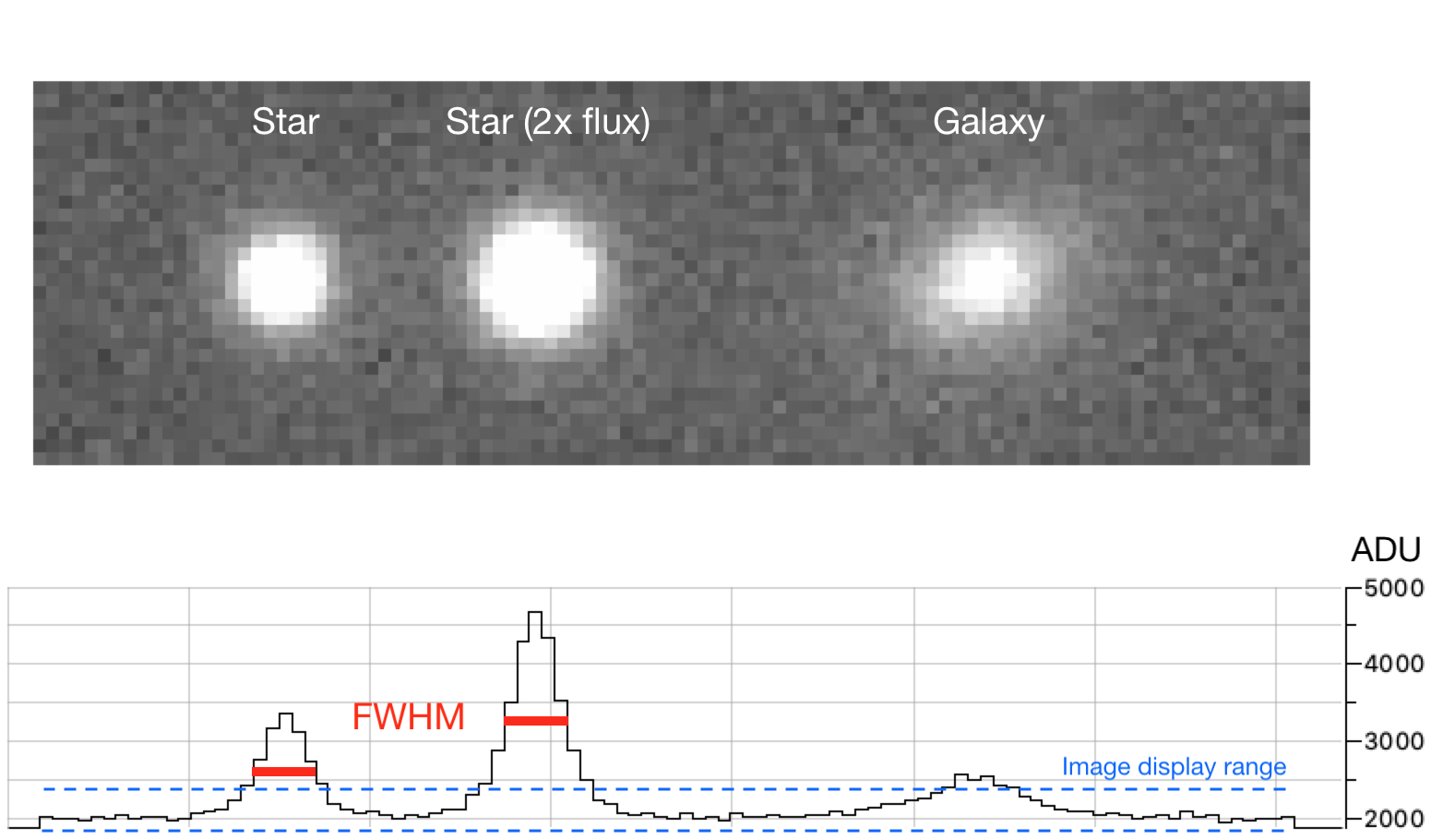
Fig. 4 Illustration of some basic image properties. Top: simulated image of two stars (one has twice the flux of the other), and one galaxy. Bottom: horizontal section across this same image, with pixel value on the y-axis. Note how the brighter star seems “larger” than the dimmer star (see text).

At this point, we can briefly discuss an image as recorded by a camera.

Recall that images of stars are not “point-like”, but follow the profile of the Point Spread Function (PSF). For images obtained by simple ground-based telescopes, the origin of the PSF is dominated by astronomical seeing, that is by refraction in bubbles of air with varying refractive index, which are rapidly moving through the line of sight due to atmospheric turbulence. The images we record through those telescopes get blurred by this PSF. Mathematically, the observed image can be seen as a convolution of the actual scene with the PSF. The result of this convolution gets sampled by the pixel array of the detector.

Also recall that the PSF is wavelength-dependent: ground-based images obtained through a red filter will be significantly sharper than images in a blue band.

Some comments about the apparent size of stars can be made:

• If two stars have a similar spectrum (or if you use a relatively narrow filter), then their profiles on the image have the same width, for example as measured by the Full Width at Half Maximum (FWHM, see Fig. 4 above) of the stars. Obviously the same holds for the standard-deviation of a 2D-Gaussian fitted to these stars, or any other measure.

• Brighter stars will have wider isophotes. An isophote is a closed curve around a star at a given brightness level. When displaying an image (i.e., when attributing a grey level to each pixel value), brighter stars will therefore appear “larger”, even if the FWHM is the same for all stars (see Fig. 4 above).

Another point illustrated in Fig. 4 is the presence of a so-called “background”, in otherwise empty areas of the image, which is here at a level of about 2000 ADU. For ground-based observations, the main source of background comes from Earth’s atmosphere: even at night, the sky is not fully dark. Light pollution, Moon light, airglow in our atmosphere, but also zodiacal light all contribute to this. When observing from Bonn at new Moon, it’s the light pollution which will dominate. Only when observing from a dark site (e.g., the Atacama desert in Chile), airglow can play the major role. In all these cases, the “background” is in fact mostly a “foreground”.

Considerations on noise

All photons falling on a pixel are subject to shot noise (also called Poisson noise), regardless of their origin from the astronomical source or the background. The same holds for the electrons from the dark current. In consequence, for any pixel, the number of recorded electrons follows a Poisson distribution, such that if the expectation value of a pixel is \(N\) electrons, the standard deviation of the noise in that pixel will be \(\sqrt{N}\) electrons. In other words, the higher the expected value of a pixel, the noisier its value will be.

Note

Be aware that this standard deviation equals \(\sqrt{N}\) only when \(N\) designates the number of electrons (or equivalently photons). This relation does not hold if \(N\) is in ADU (assuming that the gain is different from 1.0). A typical image will be stored in units of ADU, and care must be taken to convert pixel values into electrons when performing such calculations, using the gain.

The signal-to-noise ratio (S/N) quantifies how strong the level of a desired signal (for example, the flux of a galaxy) is, compared to its standard deviation. Fig. 4 illustrates how the counts from a target can actually be significantly lower than the background level. The galaxy image peaks at about 500 ADU above the background, which is at 2000 ADU. The uncertainty on the flux of this galaxy will be dominated by the shot noise from the background, more than by the shot noise from the galaxy!

Note

We’ve discussed several sources of noise: shot noise from the sources and background, shot noise from the thermal electrons (i.e., related to the dark current), and read-out noise from the electronics.

While one can easily subtract any offset or smooth model from an image, one can never subtract the actual noise.

It is therefore important to minimize noise in the first place, for example by selecting a dark observing site and cooling the camera.

FITS files

In optical astronomy, images are commonly stored in the FITS file format. We briefly introduce some nomenclature related to these FITS files, which are extensively used in the tutorial.

FITS (Flexible Image Transport System) is a standard in use since 1981, and therefore the format of choice for any long-term storage. FITS is flexible: a single file may contain several images, but also higher-dimensional arrays, data tables, or mixtures of these. Each of these entities is typically stored in a “header-data unit” (HDU). As the name implies, a HDU is composed of a “header” (holding metadata, such as the date of observation and the filter) and the actual data (such as the image). In this tutorial, we will only deal with FITS files containing a single HDU.

Interactive software for reading FITS

In the later tutorial, we will open and manipulate images stored in FITS format from within Python scripts or notebooks. While this offers exactly what we need for data analysis, it’s good to know that you can also open FITS files using programs with graphical user interfaces. For completeness, we mention here some free and multi-platform applications that are commonly used in the optical astronomy community. To visualize and inspect FITS images, you could use SAOImageDS9, often called DS9 for short. It is available on AIfA computers as ds9. An alternative is SkyCat, which was developed by the European Southern Observatory (ESO), and provides a tool to interactively “pick objects” and get, for example, centroids in sky coordinates and FWHM measurements. It’s available at the AIfA as skycat. And if you come across a FITS file containing data tables (such as a catalog of sources detected in an image), you could open and visualize its contents (and create plots) using TOPCAT, available as topcat. All these applications offer many advanced possibilities, see their respective websites for detailed descriptions and tutorials.

Calibration (aka pre-reduction)

The aim of image calibration (also known as image pre-reduction) is to remove all “artificial” or “instrumental” effects from the pixel values. Broadly speaking, these effects can be categorized as either multiplicative or additive. For example, dirt on the filter will have a multiplicative effect on the flux, as it will take away a fraction of the light of a source for certain pixels. On the other hand, the bias level is an example of an additive effect, that we want to subtract.

Image calibration attempts to cleanly separate and correct for these effects, ideally without adding any significant additional noise to the raw images. Details of an optimal pre-reduction will depend on the peculiarities of the telescopes and instruments, but the basic procedure described in the following is often part of it.

It makes use of three “calibration frames”: bias frames, dark frames, and flat frames.

Bias frames

Bias frames \(\mathbf{B}\) are frames taken with a zero exposure time. They contain the bias level, and read-out noise: all signals added by the read-out electronics.

Dark frames

Dark frames \(\mathbf{D}\) are taken with an exposure time \(t_{\mathbf{D}}\), with closed shutter, i.e., without any photons reaching the sensor. They comprise \(\mathbf{B}\), and in addition contain the thermally generated charge which increases linearly with the exposure time (integrated “dark current”). Their exposure time matters: assuming that the dark current is constant, one can use the exposure time to rescale the dark level between different exposures.

Even if the dark current might be negligible for a cooled camera, these dark frames also reveal artifacts such as hot pixels.

Flat frames

Flat frames \(\mathbf{F}\) are taken with an exposure time \(t_{\mathbf{F}}\), on an ideally uniform target. They do comprise the effects seen by \(\mathbf{B}\) and \(\mathbf{D}\), and in addition a view of the flat target contaminated by inhomogeneous sensitivity. Their purpose is to capture all multiplicative effects affecting the pixel values, such as differences in gain or quantum efficiency of the pixels, or inhomogeneous illumination of the sensor by the telescope (e.g., vignetting) or filter. Possible flatfield targets include the bright twilight sky (resulting in so-called “sky flats”), an illuminated surface inside the dome (these are called “dome flats”), or a light-emitting panel similar to a computer display (“panel flats”). Obtaining good flat frames is fundamentally difficult, as the homogeneity of a target over the full field is never perfect. Furthermore the QE variations in sensors do depend on wavelength, so that the colour (and spectrum) of the flat target matters. As will become clear, a 1% error in the flat field will yield a 1% error in the photometry of sources.

Note

Do not confuse the calibration frames and the “associated” effects! While flat frames will get used to “flatten” the pixel response across the field, they do also suffer from dark current and bias!

Science frames

We call “science frames” \(\mathbf{S}\) the actual raw exposures of the target, taken with an exposure time \(t_{\mathbf{S}}\). These images are contaminated by all the effects described in the above paragraphs.

Pre-reduction

The general idea of the pixel-by-pixel pre-reduction is to first subtract the additive effects from \(\mathbf{S}\), and then correct for the multiplicative effects through division by the flat frame. But prior to this, the latter also has to be corrected for additive effects. The overall process of the pre-reduction of \(\mathbf{S}\) can be written as follows:

\[ \mathbf{S}_{\mathrm{prered}} = \frac{\mathbf{S} - \mathbf{B} - \frac{t_{\mathbf{S}}}{t_{\mathbf{D}}}(\mathbf{D} - \mathbf{B})}{\left[\mathbf{F} - \mathbf{B} - \frac{t_{\mathbf{F}}}{t_{\mathbf{D}}}(\mathbf{D} - \mathbf{B})\right]_{\mathrm{normalized}}}, \]

where “normalized” in the denominator means that we ensure that the frame has a mean value close to one, for example by dividing it by its median pixel value. This normalization is done to avoid rescaling all pixel values in our science image by some arbitrary flat level.

In practice, instead of single bias, dark, and flat frames, one uses a masterbias, masterdark, and masterflat, i.e., combinations of several (typically 10 to 20) frames. The reason is that we don’t want to add any noise in the pre-reduction process. Combining frames (for example by taking for each pixel the median or average across several exposures) reduces the random noise compared to the signal common to the individual frames.

Note

Depending on the quality and noise of calibration frames, and on the kind of measurement one wants to perform, it can be advantageous to not calibrate, instead of performing a poor calibration.

Artifacts and dithering

• Hot pixels are defective pixels (both on CCD and CMOS sensors), which accumulate thermal electrons much faster than regular pixels. In result, when taking an image with a significant exposure time, these hot pixels will stand out as single bright points.

One simple method to mitigate the effect of such sensor artifacts is to take several “dithered” images of a target area, that is images with slightly different pointing offsets, obtained by moving the telescope by a small amount between the exposures. This ensures that the artifacts do not contaminate the targets of interest in every exposure.

Question

Why is taking several exposures usually better than taking a single exposure with a much longer exposure time?

Hint

Saturation of sources, tracking accuracy of the mount, dithering against artifacts, cosmic rays, …

Coordinates, WCS

Astronomers make use of different coordinate systems to quantify the positions of celestial objects.

On an image, the position of objects is described in pixel coordinates, that is coordinates counting pixels along the axes of the image.

On the other hand, a World Coordinate System (WCS) is a coordinate system that describes a location in “real-world units”, such as the position on the celestial sphere. The most common WCS for identifying and cataloguing sources is the equatorial system projecting the grid of terrestrial latitudes and longitudes from the centre of Earth onto the sky. The declination (Dec, \(\delta\)) is defined in analogy to latitude in geography. The (North) polar star is in approximate extension of the rotation axis of the Earth, having a declination of \(\delta = 90^{\circ}\), while the projection of the South Pole is defined to have \(\delta = -90^{\circ}\). Right ascension (RA, \(\alpha\)) is the equivalent to longitude. Its zero point is the vernal equinox point, the position of the Sun at March equinox. Both declination and right ascension are angles, but often right ascensions are expressed as times ranging from 0 hours to 24 hours, due to their close connection to the rotation of the Earth. Subsequently, subdivisions are given as time minutes and seconds rather than angular minutes and seconds!

The aim of astrometric calibration is to establish an accurate transformation between pixel coordinates and sky coordinates (e.g., RA and Dec). Such a transformation is also called “astrometric solution”. There are standard formats to write such a transformation into the header of FITS file, so that it can be very conveniently used by software tools manipulating images.

Coaddition

Once the science frames are pre-reduced and astrometrically calibrated, a possible next step is to “coadd” several exposures of a target, to obtain a deeper image revealing fainter sources. This first requires some form of reprojection of the different (dithered) images on a common pixel grid. These reprojected images can then be combined pixel-by-pixel, for example by computing an average value for each pixel across all exposures, potentially after identification and rejection of some outlier values. An alternative robust combination method is to compute the median for each pixel. While such a median-combination is easy to describe and very effective at rejecting artifacts, it is somewhat less precise than an average-combination for pixels that are not affected by any outliers. Indeed, for a large number of samples from a normal distribution, the standard error of the median will be \(\sqrt{\pi/2} \approx 1.25\) times higher, i.e., 25% greater, than the standard error of the mean (the interested reader can find details here).

In principle, it is advantageous to avoid any unnecessary manipulations to the raw data. Depending on the science case, an alternative to image coaddition is to combine the measurements obtained on the individual science frames (instead of first combining the pixel values). We will mainly follow this approach in the present tutorial.

Photometry

The brightness measurement of objects on an image is called photometry. There are two main approaches to photometry on CCD images: digital aperture photometry, and PSF fitting.

In this tutorial, we make use of digital aperture photometry, which corresponds to summing the pixel values within some aperture defined around a source (including fractional pixels, who contribute only a fraction of their value).

More specifically, we will use forced photometry, meaning that we perform photometry by placing apertures at specific pre-defined locations of an image, without first “detecting” sources in that particular image. These locations are defined in sky coordinates in a reference catalog that we build from a reference image. This makes the subsequent analysis particularly easy, as we get consistent photometric catalogs for each exposure.

In practice, photometry will deliver instrumental fluxes, measured in units of ADU, for each source (or aperture) on an exposure.

Note

For the sake of simplicity, we ignore here the effect that astrometric distortions have on photometry. For the curious: flatfielding links the pixel scale inhomogeneity of the detector to a systematic photometric bias, that in principle needs to be accounted for (either a posteriori or by reprojecting the images on a distortion-free pixel grid).

Apparent magnitudes

The apparent brightness of a source in optical astronomy, as seen in some defined passband, is denoted by an apparent magnitude in that passband. Magnitudes are a logarithmic scale of the flux that we observe from a source.

For an instrumental flux \(F\) (e.g., in ADU) obtained via photometry, one can compute an “instrumental magnitude” often defined as

\[ m_{\mathrm{instr}} = -2.5 \log_{10}(F[ADU]). \]

Clearly, this \(m_{\mathrm{instr}}\) is dependent on the instrument (and the telescope), but also on the exposure time, the aperture size, the atmospheric transparency, etc. In other words, the instrumental magnitude is a completely uncalibrated apparent magnitude, which nevertheless can be used to compare for example fluxes measured with the same observational setup.

More generally, for a source of flux \(F\) (in any appropriate unit), the magnitude is given by

\[ m = -2.5 \log_{10}(F) + C, \]

where \(C\) is a constant that calibrates the magnitude scale, often called zero point. The definition of this calibration can vary, and connecting your observations to a referential zero point can be a challenging task. In practice, this relies on the observation of standard sources whose magnitudes are known from a reference catalogue. Note that for many applications (such as the analysis of exoplanet transit light curves), an accurate magnitude calibration is not required, as we care only about relative photometry (i.e., differences in magnitudes).

Indeed, \(C\) cancels out when forming a difference in magnitudes between two sources:

\[ m_1 - m_2 = -2.5 \log_{10}\left(\frac{F_1}{F_2}\right). \]

A difference of 5 magnitudes corresponds to factor 100 in flux. Magnitude values do not have a unit, but often the word magnitude or mag is used as if it were a unit.

Note

Fainter sources have higher magnitudes!

Note

The magnitude scale is logarithmic. Any multiplicative effect on flux (such as extinction by interstellar dust, absorption by clouds, dirt on the telescope mirror, shading of parts of the telescope mirror by a misaligned dome, etc) therefore corresponds to an additive shift in magnitude, independent on the brightness of a source.

If the sources in a field would all have the same intrinsic spectrum, then any change to the passband of the instrument (i.e., using a narrower or broader filter, or a filter of a different color) would correspond to a common shift in the recorded magnitudes of all these sources.

Questions

• What flux ratio corresponds to a difference of one magnitude?

• What magnitude difference corresponds to a change in flux of \(1\%\)?

• And what about a change in flux of \(0.1\%\) (i.e., one part per thousand, or one “ppt”)?